


15
12-Lead ECG System
Augustus Désiré Waller measured the human electrocardiogram in 1887 using Lippmann's capillary electrometer (Waller, 1887). He selected five electrode locations: the four extremities and the mouth (Waller, 1889). In this way, it became possible to achieve a sufficiently low contact impedance and thus to maximize the ECG signal. Furthermore, the electrode location is unmistakably defined and the attachment of electrodes facilitated at the limb positions. The five measurement points produce altogether 10 different leads (see Fig. 15.1A). From these 10 possibilities he selected five - designated cardinal leads. Two of these are identical to the Einthoven leads I and III described below.
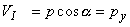
 Willem Einthoven also used the capillary electrometer in his first ECG recordings. His essential contribution to ECG-recording technology was the development and application of the string galvanometer. Its sensitivity greatly exceeded the previously used capillary electrometer. The string galvanometer itself was invented by Clément Ader (Ader, 1897). In 1908 Willem Einthoven published a description of the first clinically important ECG measuring system (Einthoven, 1908). The above-mentioned practical considerations rather than bioelectric ones determined the Einthoven lead system, which is an application of the 10 leads of Waller. The Einthoven lead system is illustrated in Figure 15.1B.
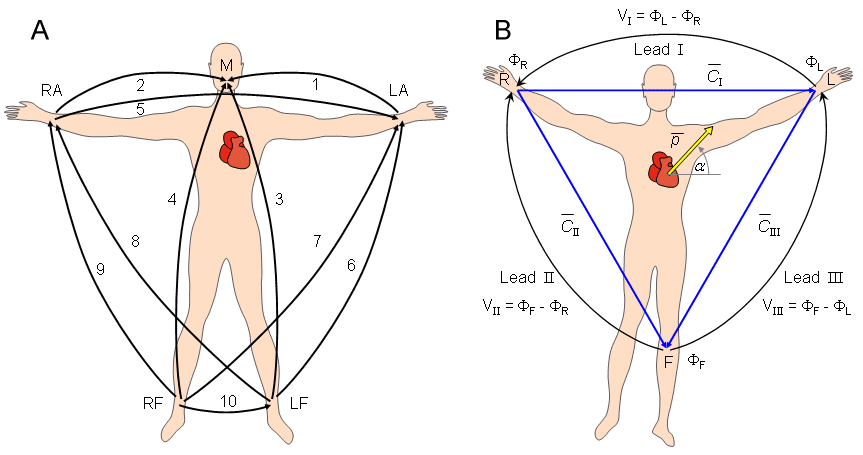
Fig. 15.1. (A) The 10 ECG leads of Waller. (B) Einthoven limb leads and Einthoven triangle. The Einthoven triangle is an approximate description of the lead vectors associated with the limb leads. Lead I is shown as  I in the above figure, etc.
The Einthoven limb leads (standard leads) are defined in the following way:
 Lead I: VI = FL - FR Lead I: VI = FL - FR | |
| Lead II: VII = FF - FR | (15.1) |
| Lead III: VIII = FF - FL |
| where | VI | = the voltage of Lead I |
| VII | = the voltage of Lead II | |
| VIII | = the voltage of Lead III | |
| FL | = potential at the left arm | |
| FR | = potential at the right arm | |
| FF | = potential at the left foot |
(The left arm, right arm, and left leg (foot) are also represented with symbols LA, RA, and LL, respectively.)
According to Kirchhoff's law these lead voltages have the following relationship:
| VI + VIII = VII | (15.2) |
hence only two of these three leads are independent.
The lead vectors associated with Einthoven's lead system are conventionally found based on the assumption that the heart is located in an infinite, homogeneous volume conductor (or at the center of a homogeneous sphere representing the torso). One can show that if the position of the right arm, left arm, and left leg are at the vertices of an equilateral triangle, having the heart located at its center, then the lead vectors also form an equilateral triangle.
A simple model results from assuming that the cardiac sources are represented by a dipole located at the center of a sphere representing the torso, hence at the center of the equilateral triangle. With these assumptions, the voltages measured by the three limb leads are proportional to the projections of the electric heart vector on the sides of the lead vector triangle, as described in Figure 15.1B. These ideas are a recapitulation of those discussed in Section 11.4.3, where it was shown that the sides of this triangle are, in fact, formed by the corresponding lead vectors.
The voltages of the limb leads are obtained from Equation 11.19, which is duplicated below (Einthoven, Fahr, and de Waart, 1913, 1950). (Please note that the equations are written using the coordinate system of the Appendix.)
 | |
 | (11.19) |
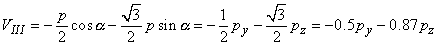 |
If one substitutes Equation 11.19 into Equation, 15.2, one can again demonstrate that Kirchhoff's law - that is, Equation 15.2 - is satisfied, since we obtain
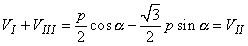 | (15.3) |
Figure 15.2 presents a volume conductor and a pair of electrodes on its opposite surfaces. The figure is divided into four cases, where both the depolarization and repolarization fronts propagate toward both positive and negative electrodes. In various cases the detected signals have the following polarities:
Case A: When the depolarization front propagates toward a positive electrode, it produces a positive signal (see the detailed description below).
Case B: When the propagation of activation is away from the positive electrode, the signal has the corresponding negative polarity.
Case C: It is easy to understand that when the repolarization front propagates toward a positive electrode, the signal is negative (see the detailed description below). Although it is known that repolarization does not actually propagate, a boundary between repolarized and still active regions can be defined as a function of time. It is "propagation" in this sense that is described here.
Case D: When the direction of propagation of a repolarization front is away from the positive electrode, a positive signal is produced.
The positive polarity of the signal in case A can be confirmed in the following way. First we note that the transmembrane voltage ahead of the wave is negative since this region is still at rest. (This condition is described in Figure 15.2 by the appearance of the minus signs.) Behind the wavefront, the transmembrane voltage is in the plateau stage; hence it is positive (indicated by the positive signs in Figure 15.2). If Equation 8.25 is applied to evaluate the double layer sources associated with this arrangement, as discussed in Section 8.2.4, and if the transmembrane voltage under resting or plateau conditions is recognized as being uniform, then a double layer source arises only at the wavefront.
What is important here is that the orientation of the double layer, given by the negative spatial derivative of Vm, is entirely to the left (which corresponds to the direction of propagation). Because the dipoles are directed toward the positive electrode, the signal is positive. (The actual time-varying signal depends on the evolving geometry of the source double layer and its relationship to the volume conductor and the leads. In this example we describe only the gross behavior.).
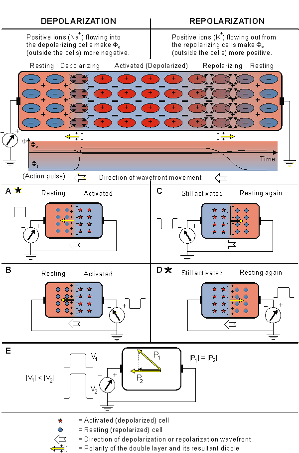
The negative polarity of the signal in case C can be confirmed in the following way. In this case the direction of repolarization allows us to designate in which regions Vm is negative (where repolarization is complete and the membrane is again at rest) and positive (where repolarization has not yet begun, and the membrane is still in the plateau stage). These are designated in Figure 15.2 by the corresponding minus (-) and plus (+) markings. In this highly idealized example, we show repolarization as occurring instantly at the - to + interface (repolarization wavefront). But the source associated with this spatial distribution of Vm is still found from Equation 8.25. Application of that equation shows that the double layer, given by the negative spatial derivative, is zero everywhere except at the repolarization wavefront, where it is oriented to the right (in this case opposite to the direction of repolarization velocity). Since the source dipoles are directed away from the positive electrode, a negative signal will be measured.
For the case that activation does not propagate directly toward an electrode, the signal is proportional to the component of the velocity in the direction of the electrode, as shown in Figure 15.2E. This conclusion follows from the association of a double layer with the activation front and application of Equation 11.4 (where we assume the direction of the lead vector to be approximated by a line connecting the leads). Note that we are ignoring the possible influence of a changing extent of the wave of activation with a change in direction. Special attention should be given to cases A and D, marked with an asterisk (*), since these reflect the fundamental relationships.
Much of what we know about the activation sequence in the heart comes from canine studies. The earliest comprehensive study in this area was performed by Scher and Young (1957). More recently, such studies were performed on the human heart, and a seminal paper describing the results was published by Durrer et al. (1970). These studies show that activation wavefronts proceed relatively uniformly, from endocardium to epicardium and from apex to base.
One way of describing cardiac activation is to plot the sequence of instantaneous depolarization wavefronts. Since these surfaces connect all points in the same temporal phase, the wavefront surfaces are also referred to as isochrones (i.e., they are isochronous). An evaluation of dipole sources can be achieved by applying generalized Equation 8.25 to each equivalent fiber. This process involves taking the spatial gradient of Vm. If we assume that on one side cells are entirely at rest, while on the other cells are entirely in the plateau phase, then the source is zero everywhere except at the wavefront. Consequently, the wavefront or isochrone not only describes the activation surface but also shows the location of the double layer sources.
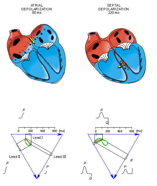
From the above it should be possible to examine the actual generation of the ECG by taking into account a realistic progression of activation double layers. Such a description is contained in Figure 15.3. After the electric activation of the heart has begun at the sinus node, it spreads along the atrial walls. The resultant vector of the atrial electric activity is illustrated with a thick arrow. The projections of this resultant vector on each of the three Einthoven limb leads is positive, and therefore, the measured signals are also positive.
After the depolarization has propagated over the atrial walls, it reaches the AV node. The propagation through the AV junction is very slow and involves negligible amount of tissue; it results in a delay in the progress of activation. (This is a desirable pause which allows completion of ventricular filling.)
Once activation has reached the ventricles, propagation proceeds along the Purkinje fibers to the inner walls of the ventricles. The ventricular depolarization starts first from the left side of the interventricular septum, and therefore, the resultant dipole from this septal activation points to the right. Figure 15.3 shows that this causes a negative signal in leads I and II.
In the next phase, depolarization waves occur on both sides of the septum, and their electric forces cancel. However, early apical activation is also occurring, so the resultant vector points to the apex.
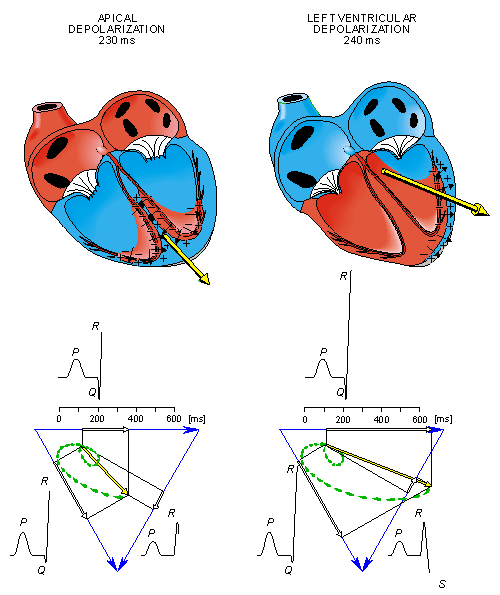
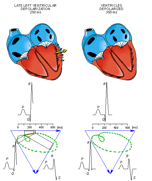
After a while the depolarization front has propagated through the wall of the right ventricle; when it first arrives at the epicardial surface of the right-ventricular free wall, the event is called breakthrough. Because the left ventricular wall is thicker, activation of the left ventricular free wall continues even after depolarization of a large part of the right ventricle. Because there are no compensating electric forces on the right, the resultant vector reaches its maximum in this phase, and it points leftward. The depolarization front continues propagation along the left ventricular wall toward the back. Because its surface area now continuously decreases, the magnitude of the resultant vector also decreases until the whole ventricular muscle is depolarized. The last to depolarize are basal regions of both left and right ventricles. Because there is no longer a propagating activation front, there is no signal either.
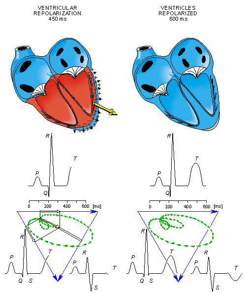
Ventricular repolarization begins from the outer side of the ventricles and the repolarization front "propagates" inward. This seems paradoxical, but even though the epicardium is the last to depolarize, its action potential durations are relatively short, and it is the first to recover. Although recovery of one cell does not propagate to neighboring cells, one notices that recovery generally does move from the epicardium toward the endocardium. The inward spread of the repolarization front generates a signal with the same sign as the outward depolarization front, as pointed out in Figure 15.2 (recall that both direction of repolarization and orientation of dipole sources are opposite). Because of the diffuse form of the repolarization, the amplitude of the signal is much smaller than that of the depolarization wave and it lasts longer.
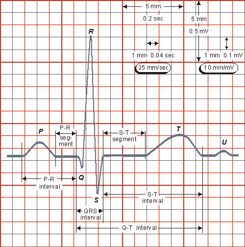
The normal electrocardiogram is illustrated in Figure 15.4. The figure also includes definitions for various segments and intervals in the ECG. The deflections in this signal are denoted in alphabetic order starting with the letter P, which represents atrial depolarization. The ventricular depolarization causes the QRS complex, and repolarization is responsible for the T-wave. Atrial repolarization occurs during the QRS complex and produces such a low signal amplitude that it cannot be seen apart from the normal ECG.
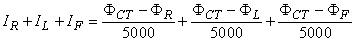
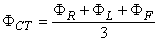
Actually, the Wilson central terminal is not independent of but, rather, is the average of the limb potentials. This is easily demonstrated by noting that in an ideal voltmeter there is no lead current. Consequently, the total current into the central terminal from the limb leads must add to zero to satisfy the conservation of current (see Figure 15.5). Accordingly, we require that
 | (15.4) |
from which it follows that
 | (15.5) |
Since the central terminal potential is the average of the extremity potentials it can be argued that it is then somewhat independent of any one in particular and therefore a satisfactory reference. In clinical practice good reproducibility of the measurement system is vital. Results appear to be quite consistent in clinical applications.
Wilson advocated 5 kW resistances; these are still widely used, though at present the high-input impedance of the ECG amplifiers would allow much higher resistances. A higher resistance increases the CMRR and diminishes the size of the artifact introduced by the electrode/skin resistance.
It is easy to show that in the image space the Wilson central terminal is found at the center of the Einthoven triangle, as shown in Figure 15.6..
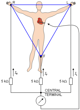
Fig. 15.5. The Wilson central terminal (CT) is formed by connecting a 5 kW resistance to each limb electrode and interconnecting the free wires; the CT is the common point. The Wilson central terminal represents the average of the limb potentials. Because no current flows through a high-impedance voltmeter, Kirchhoff's law requires that IR + IL + IF = 0.
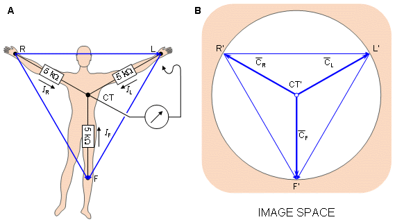
Fig. 15.6. (A) The circuit of the Wilson central terminal (CT).
(B) The location of the Wilson central terminal in the image space (CT'). It is located in the center of the Einthoven triangle.
 | (15.6) |
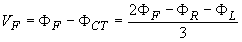
In 1942 E. Goldberger observed that these signals can be augmented by omitting that resistance from the Wilson central terminal, which is connected to the measurement electrode (Goldberger, 1942a,b). In this way, the aforementioned three leads may be replaced with a new set of leads that are called augmented leads because of the augmentation of the signal (see Figure 15.7). As an example, the equation for the augmented lead aVF is:
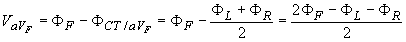 | (15.7) |
A comparison of Equation 15.7 with Equation 15.6 shows the augmented signal to be 50% larger than the signal with the Wilson central terminal chosen as reference. It is important to note that the three augmented leads, aVR, aVL, and aVF, are fully redundant with respect to the limb leads I, II, and III. (This holds also for the three unipolar limb leads VR, VL, and VF.)
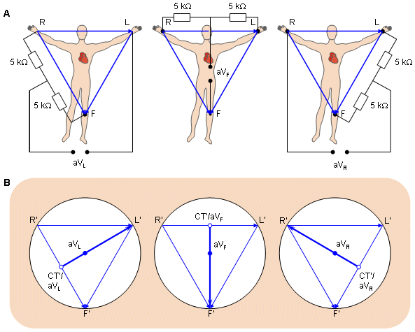
(B) The location of the Goldberger augmented lead vectors in the image space.For measuring the potentials close to the heart, Wilson introduced the precordial leads (chest leads) in 1944 (Wilson et al., 1944). These leads, V1-V6 are located over the left chest as described in Figure 15.8. The points V1 and V2 are located at the fourth intercostal space on the right and left side of the sternum; V4 is located in the fifth intercostal space at the midclavicular line; V3 is located between the points V2 and V4; V5 is at the same horizontal level as V4 but on the anterior axillary line; V6 is at the same horizontal level as V4 but at the midline. The location of the precordial leads is illustrated in Figure 15.8.
In exercise ECG, the signal is distorted because of muscular activity, respiration, and electrode artifacts due to perspiration and electrode movements. The distortion due to muscular activation can be minimized by placing the electrodes on the shoulders and on the hip instead of the arms and the leg, as suggested by R. E. Mason and I. Likar (1966). The Mason-Likar modification is the most important modification of the 12-lead system used in exercise ECG.
The accurate location for the right arm electrode in the Mason-Likar modification is a point in the infraclavicular fossa medial to the border of the deltoid muscle and 2 cm below the lower border of the clavicle. The left arm electrode is located similarly on the left side. The left leg electrode is placed at the left iliac crest. The right leg electrode is placed in the region of the right iliac fossa. The precordial leads are located in the Mason-Likar modification in the standard places of the 12-lead system.
In ambulatory monitoring of the ECG, as in the Holter recording, the electrodes are also placed on the surface of the thorax instead of the extremities.
| I, II, III | |
| aVR, aVL, aVF | |
| V1, V2, V3, V4, V5, V6 |
Of these 12 leads, the first six are derived from the same three measurement points. Therefore, any two of these six leads include exactly the same information as the other four.
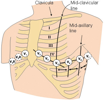
Over 90% of the heart's electric activity can be explained with a dipole source model (Geselowitz, 1964). To evaluate this dipole, it is sufficient to measure its three independent components. In principle, two of the limb leads (I, II, III) could reflect the frontal plane components, whereas one precordial lead could be chosen for the anterior-posterior component. The combination should be sufficient to describe completely the electric heart vector. (The lead V2 would be a very good precordial lead choice since it is directed closest to the x axis. It is roughly orthogonal to the standard limb plane, which is close to the frontal plane.) To the extent that the cardiac source can be described as a dipole, the 12-lead ECG system could be thought to have three independent leads and nine redundant leads.
However, in fact, the precordial leads detect also nondipolar components, which have diagnostic significance because they are located close to the frontal part of the heart. Therefore, the 12-lead ECG system has eight truly independent and four redundant leads. The lead vectors for each lead based on an idealized (spherical) volume conductor are shown in Figure 15.9. These figures are assumed to apply in clinical electrocardiography.
The main reason for recording all 12 leads is that it enhances pattern recognition. This combination of leads gives the clinician an opportunity to compare the projections of the resultant vectors in two orthogonal planes and at different angles. This is further facilitated when the polarity of the lead aVR can be changed; the lead -aVR is included in many ECG recorders.
In summary, for the approximation of cardiac electric activity by a single fixed-location dipole, nine leads are redundant in the 12-lead system, as noted above. If we take into account the distributed character of cardiac sources and the effect of the thoracic surface and internal inhomogeneities, we can consider only the four (of six) limb leads as truly redundant..
Fig. 15.9. The projections of the lead vectors of the 12-lead ECG system in three orthogonal planes when one assumes the volume conductor to be spherical homogeneous and the cardiac source centrally located.
Ader C (1897): Sur un nouvel appareil enregistreur pour cables sousmarins. Compt. rend. Acad. Sci. (Paris) 124: 1440-2.
Durrer D, van Dam RT, Freud GE, Janse MJ, Meijler FL, Arzbaecher RC (1970): Total excitation of the isolated human heart. Circulation 41:(6) 899-912.
Einthoven W (1908): Weiteres über das Elektrokardiogram. Pflüger Arch. ges. Physiol. 122: 517-48.
Einthoven W, Fahr G, de Waart A (1913): Über die Richtung und die Manifeste Grösse der Potentialschwankungen im mennschlichen Herzen und über den Einfluss der Herzlage auf die form des Elektrokardiogramms. Pflüger Arch. ges. Physiol. 150: 275-315.
Einthoven W, Fahr G, de Waart A (1950): On the direction and manifest size of the variations of potential in the human heart and on the influence of the position of the heart on the form of the electrocardiogram. Am. Heart J. 40:(2) 163-211. (Reprint 1913, translated by HE Hoff, P Sekelj).
Geselowitz DB (1964): Dipole theory in electrocardiography. Am. J. Cardiol. 14:(9) 301-6.
Goldberger E (1942a): The aVL, aVR, and aVF leads; A simplification of standard lead electrocardiography. Am. Heart J. 24: 378-96.
Goldberger E (1942b): A simple indifferent electrocardiographic electrode of zero potential and a technique of obtaining augmented, unipolar extremity leads. Am. Heart J. 23: 483-92.
Mason R, Likar L (1966): A new system of multiple leads exercise electrocardiography. Am. Heart J. 71:(2) 196-205.
Netter FH (1971): Heart, Vol. 5, 293 pp. The Ciba Collection of Medical Illustrations, Ciba Pharmaceutical Company, Summit, N.J.
Scher AM, Young AC (1957): Ventricular depolarization and the genesis of the QRS. Ann. N.Y. Acad. Sci. 65: 768-78.
Waller AD (1887): A demonstration on man of electromotive changes accompanying the heart's beat. J. Physiol. (Lond.) 8: 229-34.
Waller AD (1889): On the electromotive changes connected with the beat of the mammalian heart, and on the human heart in particular. Phil. Trans. R. Soc. (Lond.) 180: 169-94.
Wilson FN, Johnston FD, Macleod AG, Barker PS (1934): Electrocardiograms that represent the potential variations of a single electrode. Am. Heart J. 9: 447-71.
Wilson FN, Johnston FD, Rosenbaum FF, Erlanger H, Kossmann CE, Hecht H, Cotrim N, Menezes de Olivieira R, Scarsi R, Barker PS (1944): The precordial electrocardiogram. Am. Heart J. 27: 19-85.
Wilson FN, Macleod AG, Barker PS (1931): Potential variations produced by the heart beat at the apices of Einthoven's triangle. Am. Heart J. 7: 207-11.
Macfarlane PW, Lawrie TDV (eds.) (1989): Comprehensive Electrocardiology: Theory and Practice in Health and Disease, 1st ed., Vol. 1, 2, and 3, 1785 pp. Pergamon Press, New York.
Nelson CV, Geselowitz DB (eds.) (1976): The Theoretical Basis of Electrocardiology, 544 pp. Oxford University Press, Oxford.
Pilkington TC, Plonsey R (1982): Engineering Contributions to Biophysical Electrocardiography, 248 pp. IEEE Press, John Wiley, New York.