


3
Subthreshold membrane phenomena
In the previous chapter the subthreshold behavior of the nerve cell was discussed qualitatively. This chapter describes the physiological basis of the resting voltage and the subthreshold response of an axon to electric stimuli from a quantitative perspective.
 We = Q(FP - FO) We = Q(FP - FO) | (3.1) |
| where | We | = work [J/mol] |
| Q | = charge [C] (coulombs) | |
| F | = potential [V] |
In electrophysiological problems the quantity of ions is usually expressed in moles. (One mole equals the molecular weight in grams-hence 6.0225 × 10˛ł, Avogadro's number of molecules.) If one mole of an ion is transferred from a reference point O at potential FO to an arbitrary point P at potential FP, then from Equation 3.1 the required work is
| We = zF(FP - FO) | (3.2) |
| where | We | = work [J/mol] |
| z | = valence of the ions | |
| F | = Faraday's constant [9.649 × 10⁴ C/mol] | |
| F | = potential [V] |
Faraday's constant converts quantity of moles to quantity of charge for a univalent ion. The factor z, called valence, takes into account multivalent ions and also introduces the sign. Note that if FP - FO and z are both positive (i.e., the case where a positive charge is moved from a lower to higher potential), then work must be done, and We is positive as expected.
 , then the work done against the electric field force
  , according to the basic laws of mechanics, is the work dW given by
 | (3.3) |
Applying Equation 3.1 to Equation 3.3 (replacing Q by unity) gives:
 | (3.4) |
The Taylor series expansion of the scalar field about the point O and along the path s is:
| FP = FO dF/ds + ··· | (3.5) |
Since P is very close to O, the remaining higher terms may be neglected in Equation 3.5. The second term on the right-hand side of Equation 3.5 is known as the directional derivative of F in the direction s. The latter, by the vector-analytic properties of the gradient, is given by  . Consequently, Equation 3.5 may be written as
 | (3.6) |
From Equations 3.4 and 3.6 we deduce that
 | (3.7) |
This relationship is valid not only for electrostatics but also for electrophysiological problems since quasistatic conditions are known to apply to the latter (see Section 8.2.2).
 and electric field are related by
 | (3.8) |
where s is the conductivity of the medium. This current, for obvious reasons, is called a conduction current.
 | (3.9) |
| where |  ke ke | = ionic flux (due to electric field) [mol/(cm˛·s)] |
| uk | = ionic mobility [cm˛/(V·s)] | |
| zk | = valence of the ion | |
| ck | = ionic concentration [mol/cmł] |
and further:
 | = | the sign of the force (positive for cations and negative for anions) | |
 | = | the mean velocity achieved by these ions in a unit electric field (according to the definition of uk) | |
| the subscript k denotes the kth ion. |
Multiplying ionic concentration ck by velocity gives the ionic flux. A comparison of Equation 3.8 with Equation 3.9 shows that the mobility is proportional to the conductivity of the kth ion in the electrolyte. The ionic mobility depends on the viscosity of the solvent and the size and charge of the ion.
 | (3.10) |
| where | kD | = ionic flux (due to diffusion) [mol/(cm˛·s)] |
| Dk | = Fick's constant (diffusion constant) [cm˛/s] | |
| ck | = ion concentration [mol/cmł] |
This equation describes flux in the direction of decreasing concentration (accounting for the minus sign), as expected.
 ck ) to the consequent flux of the kth substance. In a similar way the mobility couples the electric field force (-F) to the resulting ionic flux. Since in each case the flux is limited by the same factors (collision with solvent molecules), a connection between uk and Dk should exist. This relationship was worked out by Nernst (1889) and Einstein (1905) and is
 | (3.11) |
| where | T | = absolute temperature [K] |
| R | = gas constant [8.314 J/(mol·K)] |
k , is given by the sum of ionic fluxes due to diffusion and electric field of Equations 3.10 and 3.9. Using the Einstein relationship of Equation 3.11, it can be expressed as
 | (3.12) |
Equation 3.12 is known as the Nernst-Planck equation (after Nernst, 1888, 1889; Planck, 1890ab). It describes the flux of the kth ion under the influence of both a concentration gradient and an electric field. Its dimension depends on those used to express the ionic concentration and the velocity. Normally the units are expressed as [mol/(cm˛·s)].
can be converted into an electric current density by multiplying the former by zF, the number of charges carried by each mole (expressed in coulombs, [C]). The result is, for the kth ion,
 | (3.13) |
| where | k | = electric current density due to the kth ion [C/(s·cm˛)] = [A/cm˛] |
Using Equation 3.11, Equation 3.13 may be rewritten as
 | (3.14) |
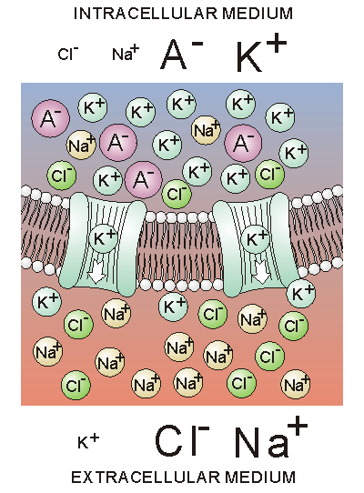
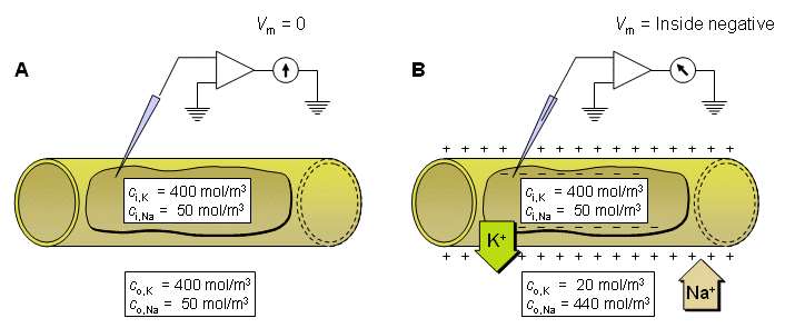
Fig. 3.1. A patch of membrane of an excitable cell at rest with part of the surrounding intracellular and extracellular media. The main ions capable of transmembrane flow are potassium (K+), sodium (Na+), and chloride (Cl-). The intracellular ionic composition and extracellular ionic composition are unequal. At the sides of the figure, the sizes of the symbols reflect the proportions of the corresponding ion concentration. The intracellular anion (A-) is important to the achievement of electroneutrality; however, A- is derived from large immobile and impermeable molecules (KA), and thus A- does not contribute to ionic flow. At rest, the membrane behaves as if it were permeable only to potassium. The ratio of intracellular to extracellular potassium concentration is in the range 30-50:1. (The ions and the membrane not shown in scale.)
 | (3.15) |
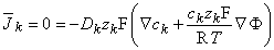
where the subscript k refers to an arbitrary kth ion. Transposing terms in Equation 3.15 gives
 | (3.16) |
Since the membrane is extremely thin, we can consider any small patch as planar and describe variations across it as one-dimensional (along a normal to the membrane). If we call this direction x, we may write out Equation 3.16 as
 | (3.17) |
Equation 3.17 can be rearranged to give
 | (3.18) |
Equation 3.18 may now be integrated from the intracellular space (i) to the extracellular space (o); that is:
 | (3.19) |
Carrying out the integrations in Equation 3.19 gives
 | (3.20) |
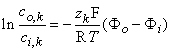
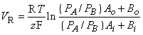
where ci,k and co,k denote the intracellular and extracellular concentrations of the kth ion, respectively. The equilibrium voltage across the membrane for the kth ion is, by convention, the intracellular minus the extracellular potential (Vk = Fi - Fo), hence:
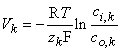 | (3.21) |
| where | Vk | = equilibrium voltage for the kth ion across the membrane Fi - Fo i.e., the Nernst voltage [V] |
| R | = gas constant [8.314 J/(mol·K)] | |
| T | = absolute temperature [K] | |
| zk | = valence of the kth ion | |
| F | = Faraday's constant [9.649 × 10⁴ C/mol] | |
| ci,k | = intracellular concentration of the kth ion | |
| co,k | = extracellular concentration of the kth ion |
Equation 3.21 is the famous Nernst equation derived by Walther Hermann Nernst in 1888 (Nernst, 1888). By Substituting 37 °C which gives T = 273 + 37 and +1 for the valence, and by replacing the natural logarithm (the Napier logarithm) with the decadic logarithm (the Briggs logarithm), one may write the Nernst equation for a monovalent cation as:
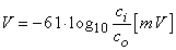 | (3.22) |
At room temperature (20 °C), the coefficient in Equation 3.22 has the value of 58; at the temperature of seawater (6 °C), it is 55. The latter is important when considering the squid axon.
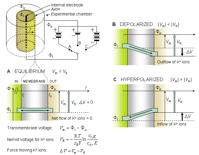
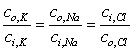
Fig. 3.2. An example illustrating the Nernst equation and ion flow through the membrane in
 | (3.23) |
Note that Equation 3.23 reflects the fact that all ions are univalent and that chloride is negative. The condition represented by Equation 3.23 is that all ions are in equilibrium; it is referred to as the Donnan equilibrium.
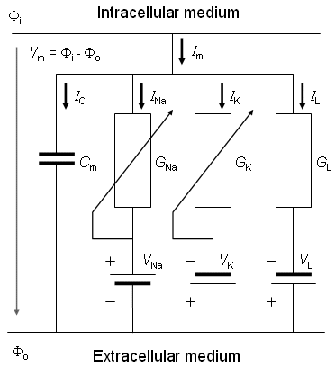
Fig. 3.4. An electric circuit representation of a membrane patch. In this diagram, VNa, VK, and VL represent the absolute values of the respective emf's and the signs indicate their directions when the extracellular medium has a normal composition (high Na and Cl, and low K, concentrations).
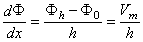 | (3.24) |
| where | F0 | = potential at the outer membrane surface |
| Fh | = potential at the inner membrane surface | |
| Vm | = transmembrane voltage | |
| h | = membrane thickness |
This approximation was originally introduced by David Goldman (1943).
 ,
,  , and, using Equation 3.12, we get
 | (3.25) |
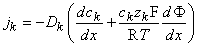
for the kth ion flux. If we now insert the constant field approximation of Equation 3.24 (dF/dx = Vm/h) the result is
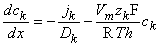 | (3.26) |
(To differentiate ionic concentration within the membrane from that outside the membrane (i.e., inside versus outside the membrane), we use the symbol cm in the following where intramembrane concentrations are indicated.) Rearranging Equation 3.26 gives the following differential equation:
 | (3.27) |
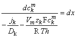
We now integrate Equation 3.27 within the membrane from the left-hand edge (x = 0) to the right-hand edge (x = h). We assume the existence of resting conditions; hence each ion flux must be in steady state and therefore uniform with respect to x. Furthermore, for Vm to remain constant, the total transmembrane electric current must be zero. From the first condition we require that jk(x) be a constant; hence on the left-hand side of Equation 3.27, only ckm(x) is a function of x. The result of the integration is then
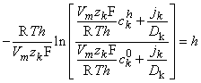 | (3.28) |
| where | ckh | = concentration of the kth ion at x = h |
| ck0 | = concentration of the kth ion at x = 0 |
Equation 3.28 can be solved for jk, giving
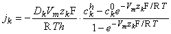 | (3.29) |
The concentrations of the kth ion in Equation 3.29 are those within the membrane. However, the known concentrations are those in the intracellular and extracellular (bulk) spaces. Now the concentration ratio from just outside to just inside the membrane is described by a partition coefficient, b. These are assumed to be the same at both the intracellular and extracellular interface. Consequently, since x = 0 is at the extracellular surface and x = h the intracellular interface, we have
  | (3.30) |
| where | b | = partition coefficient |
| ci | = measurable intracellular ionic concentration | |
| co | = measurable extracellular ionic concentration |
 | (3.31) |
then
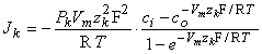 | (3.32) |
 | (3.33) |
 | (3.34) |
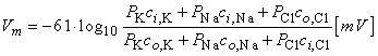
In Equation 3.34 the expression for sodium ion current is seen to be similar to that for potassium (except for exchanging Na for K); however, the expression for chloride requires, in addition, a change in sign in the exponential term, a reflection of the negative valence.
 | (3.35) |
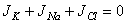
Multiplying through by the permeabilities and collecting terms gives:
 | (3.36) |
From this equation, it is possible to solve for the potential difference Vm across the membrane, as follows:
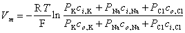 | (3.37) |
where Vm evaluates the intracellular minus extracellular potential (i.e., transmembrane voltage). This equation is called the Goldman-Hodgkin-Katz equation. Its derivation is based on the works of David Goldman (1943) and Hodgkin and Katz (1949). One notes in Equation 3.37 that the relative contribution of each ion species to the resting voltage is weighted by that ion's permeability. For the squid axon, we noted (Section 3.5.2) that PNa/PK = 0.04, which explains why its resting voltage is relatively close to VK and quite different from VNa.
 | (3.38) |
Example
It is easy to demonstrate that the Goldman-Hodgkin-Katz equation (Equation 3.37) reduces to the Nernst equation (Equation 3.21). Suppose that the chloride concentration both inside and outside the membrane were zero (i.e., co,Cl = ci,Cl = 0). Then the third terms in the numerator and denominator of Equation 3.37 would be absent. Suppose further that the permeability to sodium (normally very small) could be taken to be exactly zero (i.e., PNa = 0). Under these conditions the Goldman-Hodgkin-Katz equation reduces to the form of the Nernst equation (note that the absolute value of the valence of the ions in question |z| = 1). This demonstrates again that the Nernst equation expresses the equilibrium potential difference across an ion permeable membrane for systems containing only a single permeable ion.
 | (3.39) |
This equation resembles the Nernst equation (Equation 3.21), but it includes two types of ions. It is the simplest form of the Goldman-Hodgkin-Katz equation (Equation 3.37).
For each ion, the following equilibrium voltages may be calculated from the Nernst equation:
The resting voltage of the cell was measured to be -70 mV.
We further define the currents and voltages of the circuit as follows (see Figures 3.6 and 3.7):
A graphical sketch defining of various potentials and voltages in the axon is given in Figure 3.8.
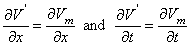
In the special case when there are no stimulating currents (i.e., when Ii = Io = Im = 0), then Vm = Vr and V' = 0. However, once activation has been initiated we shall see that it is possible for Ii + Io = 0 everywhere and V'
based on the definition of V' given above.
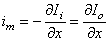
From the current conservation laws, it follows also that the transmembrane current per unit length, im, must be related to the loss of Ii or to the gain of Io as follows:
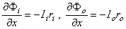
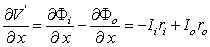
Note that this expression is consistent with Ii + Io = 0. The selection of the signs in Equation 3.42 is based on outward-flowing current being defined as positive. From these definitions and Equations 3.40 and 3.41 (and recalling that V' = Fi - Fo - Vr), it follows that
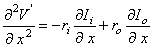
Furthermore, by differentiating with respect to x, we obtain:
Substituting Equation 3.42 into Equation 3.44 gives:
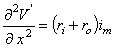
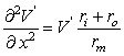
which is called the general cable equation.
whose solution is
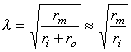
The constant l in Equation 3.47 has the dimension of length and is called the characteristic length or length constant of the axon. It is called also the space constant. The characteristic length l is related to the parameters of the axon by Equation 3.46, and is given by:
The latter form of Equation 3.48 may be written because the extracellular axial resistance ro is frequently negligible when compared to the intracellular axial resistance ri.
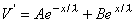
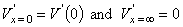
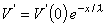
the constants A and B take on the values A = V'(0) and B = 0, and from Equation 3.47 we obtain the solution:
This expression indicates that V' decreases exponentially along the axon beginning at the point of stimulation (x = 0), as shown in Figure 3.9B. At x = l the amplitude has diminished to 36.8% of the value at the origin. Thus l is a measure of the distance from the site of stimulation over which a significant response is obtained. For example at x = 2l the response has diminished to 13.5%, whereas at x = 5l it is only 0.7% of the value at the origin.
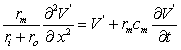
The left side of Equation 3.51 evaluates the total membrane current im, whereas on the right side the first term represents the resistive component (formed by the ionic currents), and the second term the capacitive current which must now be included since
which can be easily expressed as
where t = rmcm is the time constant of the membrane and l is the space constant as defined in Equation 3.48.
Fig. 3.10. The response of the axon to a step-current impulse.
Fig. 3.11. Subthreshold transmembrane voltage response to a step current of very long duration at different instants of time (upper graphs) and at different distances from the sites of stimulation (lower graphs). The responses when the current is turned on and off are shown in the left and right sides of the figure, respectively.
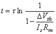
Fig. 3.12. The derivation of the strength-duration curve.
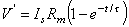
The membrane is assumed to be activated if its voltage reaches the threshold value. We consider this condition if we substitute V' = DVth into Equation 3.56, where Vth is the change in the resting voltage needed just to reach the threshold voltage. Equation 3.56 may now be written in the form:
Fig. 3.13. (A) Strength-duration curve. The units are relative.
The analytical results above are approximate for several reasons. First, the excitable tissue cannot normally be well approximated by a lumped R since such elements are actually distributed. (In a space-clamp stimulation the membrane can be more accurately represented with a lumped model.) Also the use of a linear model is satisfactory up to perhaps 80% of the threshold, but beyond this the membrane behaves nonlinearly. Another approximation is the idea of a fixed threshold; in a subsequent chapter, we describe accommodation, which implies a threshold rising with time.
3.5 ION FLOW THROUGH THE MEMBRANE
3.5.1 Factors Affecting Ion Transport Through the Membrane
This section explores the flow of various ions through the membrane under normal resting conditions.
3.5.2 Membrane Ion Flow in a Cat Motoneuron
We discuss the behavior of membrane ion flow with an example. For the cat motoneuron the following ion concentrations have been measured (see Table 3.1).
Outside
Inside
Na+ 150 15 K+ 5.5 150
Cl- 125 9
Chloride Ions
In this example the equilibrium potential of the chloride ion is the same as the resting potential of the cell. While this is not generally the case, it is true that the chloride Nernst potential does approach the resting potential. This condition arises because chloride ion permeability is relatively high, and even a small movement into or out of the cell will make large changes in the concentration ratios as a result of the very low intracellular concentration. Consequently the concentration ratio, hence the Nernst potential, tends to move toward equilibrium with the resting potential.
Potassium ions
In the example described by Table 3.1, the equilibrium voltage of potassium is 19 mV more negative than the resting voltage of the cell. In a subsequent section we shall explain that this is a typical result and that the resting potential always exceeds (algebraically) the potassium Nernst potential. Consequently, we must always expect a net flow of potassium ions from the inside to the outside of a cell under resting conditions. To compensate for this flux, and thereby maintain normal ionic composition, the potassium ion must also be transported into the cell. Such a movement, however, is in the direction of increasing potential and consequently requires the expenditure of energy. This is provided by the Na-K pump,that functions to transport potassium at the expense of energy.
Sodium Ions
The equilibrium potential of sodium is +61 mV, which is given by the concentration ratio (see Table 3.1). Consequently, the sodium ion is 131 mV from equilibrium, and a sodium influx (due to both diffusion and electric field forces) will take place at rest. Clearly neither sodium nor potassium is in equilibrium, but the resting condition requires only a steady-state. In particular, the total membrane current has to be zero. For sodium and potassium, this also means that the total efflux and total influx must be equal in magnitude. Since the driving force for sodium is 6.5 times greater than for potassium, the potassium permeability must be 6.5 times greater than for sodium. Because of its low resting permeability, the contribution of the sodium ion to the resting transmembrane potential is sometimes ignored, as an approximation.
3.5.3 Na-K Pump
The long-term ionic composition of the intracellular and extracellular space is maintained by the Na-K pump. As noted above, in the steady state, the total passive flow of electric current is zero, and the potassium efflux and sodium influx are equal and opposite (when these are the only contributing ions). When the Na-K pump was believed to exchange 1 mol potassium for 1 mol sodium, no net electric current was expected. However recent evidence is that for 2 mol potassium pumped in, 3 mol sodium is pumped out. Such a pump is said to be electrogenic and must be taken into account in any quantitative model of the membrane currents (Junge, 1981).
3.5.4 Graphical Illustration of the Membrane Ion Flow
The flow of potassium and sodium ions through the cell membrane (shaded) and the electrochemical gradient causing this flow are illustrated in Figure 3.5. For each ion the clear stripe represents the ion flux; the width of the stripe, the amount of the flux; and the inclination (i.e., the slope), the strength of the electrochemical gradient.
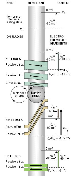
Fig. 3.5. A model illustrating the transmembrane ion flux. (After Eccles, 1968.) (Note that for K+ and Cl- passive flux due to diffusion and electric field are shown separately)
3.6 CABLE EQUATION OF THE AXON
Ludvig Hermann (1905b) was the first to suggest that under subthreshold conditions the cell membrane can be described by a uniformly distributed leakage resistance and parallel capacitance. Consequently, the response to an arbitrary current stimulus can be evaluated from an elaboration of circuit theory. In this section, we describe this approach in a cell that is circularly cylindrical in shape and in which the length greatly exceeds the radius. (Such a model applies to an unmyelinated nerve axon.)
3.6.1 Cable Model of the Axon
Suppose that an axon is immersed in an electrolyte of finite extent (representing its extracellular medium) and an excitatory electric impulse is introduced via two electrodes - one located just outside the axon in the extracellular medium and the other inside the axon, as illustrated in Figure 3.6. The total stimulus current (Ii), which flows axially inside the axon, diminishes with distance since part of it continually crosses the membrane to return as a current (Io) outside the axon. Note that the definition of the direction of positive current is to the right for both Ii and Io, in which case conservation of current requires that Io = -Ii. Suppose also that both inside and outside of the axon, the potential is uniform within any crossection (i.e., independent of the radial direction) and the system exhibits axial symmetry. These approximations are based on the cross-sectional dimensions being very small compared to the length of the active region of the axon. Suppose also that the length of the axon is so great that it can be assumed to be infinite.
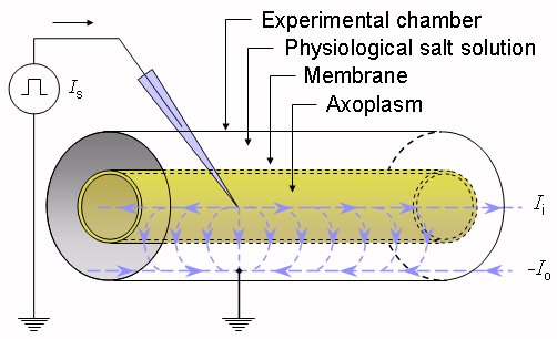
Fig. 3.6. The experimental arrangement for deriving the cable equation of the axon.
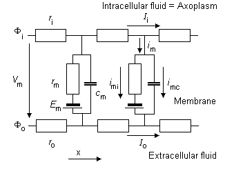
Fig. 3.7. The equivalent circuit model of an axon. An explanation of the component elements is given in the text.
ri = intracellular axial resistance of the axoplasm per unit length of axon [kW/cm axon length] ro = extracellular axial resistance of the (bounding) extracellular medium per unit length of axon [kW/cm axon length]
rm = membrane resistance times unit length of axon [kW·cm axon length] (note that this is in the radial direction, which accounts for its dimensions) cm = membrane capacitance per unit length of axon [µF/cm axon length]
Ii = total longitudinal intracellular current [µA] Io = total longitudinal extracellular current [µA] im = total transmembrane current per unit length of axon [µA/cm axon length] (in radial direction) imC = capacitive component of the transmembrane current per unit length of axon [µA/cm axon length] imI = ionic component of the transmembrane current per unit length of axon [µA/cm axon length] Fi = potential inside the membrane [mV] Fo = potential outside the membrane [mV] Vm = Fi - Fo membrane voltage [mV] Vr = membrane voltage in the resting state [mV] V' = Vm - Vr = deviation of the membrane voltage from the resting state [mV] 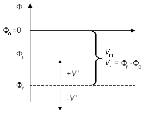
Fig. 3.8. A graphical sketch depicting various potentials and voltages in the axon used in this book.
 0 in certain regions.
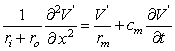
(3.40) 3.6.2 The Steady-State Response
We first consider the stationary case (i.e., d/dt = 0) which is the steady-state condition achieved following the application of current step. This corresponds to the limit t 
 . The steady-state response is illustrated in Figure 3.9. It follows from Ohm's law that
(3.41)
(3.42)
(3.43)
(3.44) 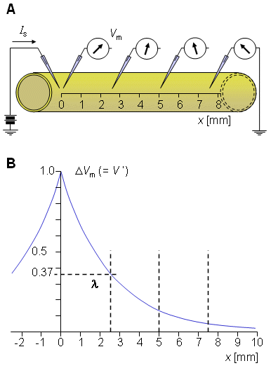
Fig. 3.9. (A) Stimulation of a nerve with current step.
(3.45)
(3.46)
(3.47)
(3.48)
(3.49) 3.6.3 Stimulation with a Step-Current Impulse
In this section we consider the transient (rather than steady-state) response of the axon to a subthreshold current-step input. In this case the membrane current is composed of both resistive and capacitive components reflecting the parallel RC nature of the membrane:

(3.50)
where im = the total membrane current per unit length [µA/cm axon length] imR = the resistive component of the membrane current per unit length [µA/cm axon length] imC = the capacitive component of the membrane current per unit length [µA/cm axon length]
(3.51)  /t 0 . Equation 3.51 may also be written in the form:
(3.52)
(3.53) 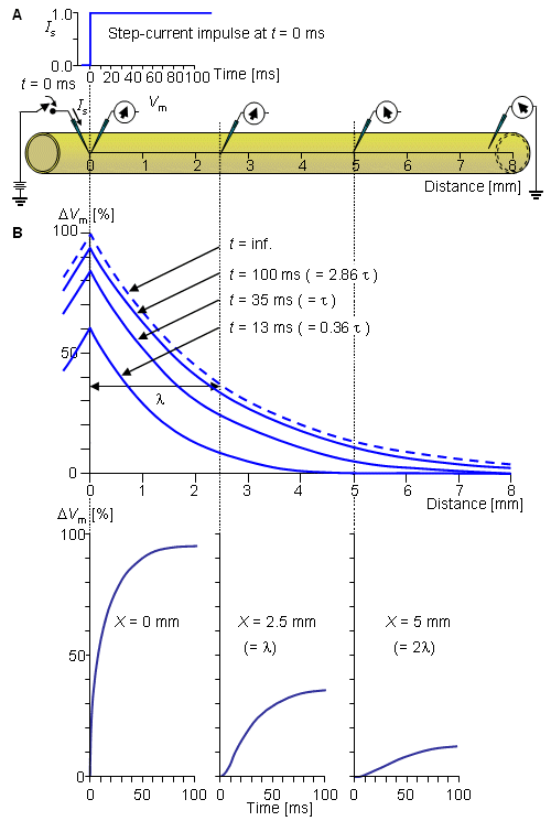 . The latter curve is the steady-state response and corresponds to Equation 3.49.
Quantity Dimension Species Squid Lobster Crayfish
diameter [µm] 500 75 30 characteristic length l [cm] 0.5 0.25 0.25 time constant t [ms] 0.5 0.25 0.25 specific resistance of the membrane *) [kW·cm2] 0.7 2.0 5.0 specific capacitance of the membrane *) [µF/cm2] 1 1 1 *) The specific resistance and specific capacitance of the membrane can be calculated from values of
Rm = 2parm(3.54) Cm = cm/(2pa)(3.55)
where Rm = specific resistance of the membrane (membrane resistance times unit area) [kW·cm2] rm = membrane resistance times unit length [kW·cm axon length] Cm = specific capacitance of the membrane (membrane capacitance per unit area) [µF/cm˛] cm = membrane capacitance per unit length [µF/cm axon length] a = fiber radius [cm]. 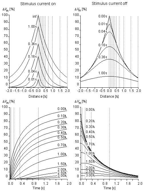
3.7 STRENGTH-DURATION RELATION
When an excitable membrane is depolarized by a stimulating current whose magnitude is gradually increased, a current level will be reached, termed the threshold, when the membrane undergoes an action impulse. The latter is characterized by a rapid and phasic change in membrane permeabilities, and associated transmembrane voltage. An illustration of this process was given in Figure 2.8, where the response to stimulus level 2 is subthreshold, whereas stimulus 3 appears just at threshold (since sometimes an action potential (3B) results whereas at other times a passive response (3A) is observed). An action potential is also clearly elicited for the transthreshold stimulus of 4.
(3.56)
where V' = change in the membrane voltage [mV] Is = stimulus current per unit area [µA/cm˛] Rm = membrane resistance times unit area [kW·cm˛] t = stimulus time [ms] t = membrane time constant = RmCm [ms] Cm = membrane capacitance per unit surface [µF/cm˛] 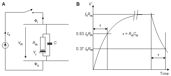
(3.57)

(3.58)
(3.59)
(3.60)
(3.61)
(3.62) 
Tissue Time [ms] Skeletal muscle
Frog (gastrocnemius)
Frog (sartorius
Turtle (leg flexors and extensors)
Man (arm flexors)
Man (arm extensors)
Man (thigh muscles)
Man (facial muscles)
0.2-0.3
0.3
1-2
0.08-0.1
0.16-0.3
0.10-0.7
0.24-0.7
Cardiac muscle
Frog (ventricle)
Turtle (ventricle)
Dog (ventricle)
Man (ventricle)
3
2
2
2
Smooth muscle
Frog (stomach)
100
Nerve
Frog (sciatic)
Man (A fibers)
Man (vestibular)
0.3
0.2
14-22
Receptors
Man (tongue)
Man (retinal rods)
Man (retinal cones)
1.4-1.8
1.2-1.8
2.1-3.0
Arvanitaki A (1938): Les Variations Graduées De La Polarisation Des Systčmes Excitables, Hermann, Paris.
Bernstein J (1902): Untersuchungen zur Termodynamik der bioelektrischen Ströme. Pflüger Arch. ges. Physiol. 9: 521-62.
Bernstein J (1912): Elektrobiologie, 215 pp. Viewag, Braunschweig.
Davis LJ, Lorente de Nó R (1947): Contributions to the mathematical theory of the electrotonus. Stud. Rockefeller Inst. Med. Res. 131: 442-96.
Eccles JC (1968): The Physiology of Nerve Cells, 270 pp. The Johns Hopkins Press, Baltimore.
Einstein A (1905): Über die von der molekularkinetischen Theorie die wärme Gefordertebewegung von in ruhenden flüssigkeiten suspendierten Teilchen. Ann. Physik 17: 549-60.
Faraday M (1834): Experimental researches on electricity, 7th series. Phil. Trans. R. Soc. (Lond.) 124: 77-122.
Fick M (1855): Über Diffusion. Ann. Physik und Chemie 94: 59-86.
Goldman DE (1943): Potential, impedance, and rectification in membranes. J. Gen. Physiol. 27: 37-60.
Hermann L (1905): Beiträge zur Physiologie und Physik des Nerven. Pflüger Arch. ges. Physiol. 109: 95-144.
Hille B (1992): Ionic Channels of Excitable Membranes, 2nd ed., 607 pp. Sinauer Assoc., Sunderland, Mass. (1st ed., 1984)
Hodgkin AL, Huxley AF (1952): A quantitative description of membrane current and its application to conduction and excitation in nerve. J. Physiol. (Lond.) 117: 500-44.
Hodgkin AL, Huxley AF, Katz B (1952): Measurement of current-voltage relations in the membrane of the giant axon of Loligo. J. Physiol. (Lond.) 116: 424-48.
Hodgkin AL, Katz B (1949): The effect of sodium ions on the electrical activity of the giant axon of the squid. J. Physiol. (Lond.) 108: 37-77.
Hodgkin AL, Rushton WA (1946): The electrical constants of a crustacean nerve fiber. Proc. R. Soc. (Biol.) B133: 444-79.
Katchalsky A, Curran PF (1965): Nonequilibrium Thermodynamics in Biophysics, 248 pp. Harvard University Press, Cambridge, Mass.
Kortum G (1965): Treatise on Electrochemistry, 2nd ed., 637 pp. Elsevier, New York.
Nernst WH (1888): Zur Kinetik der Lösung befindlichen Körper: Theorie der Diffusion. Z. Phys. Chem. 3: 613-37.
Nernst WH (1889): Die elektromotorische Wirksamkeit der Ionen. Z. Phys. Chem. 4: 129-81.
Planck M (1890a): Über die Erregung von Elektricität und Wärme in Elektrolyten. Ann. Physik und Chemie, Neue Folge 39: 161-86.
Planck M (1890b): Über die Potentialdifferenz zwischen zwei verdünnten Lösungen binärer Elektrolyte. Ann. Physik und Chemie, Neue Folge 40: 561-76.
Ruch TC, Patton HD (eds.) (1982): Physiology and Biophysics, 20th ed., 1242 pp. W. B. Saunders, Philadelphia.
Rysselberghe van P (1963): Thermodynamics of Irreversible Processes, 165 pp. Hermann, Paris, and Blaisedell, New York.
Edsall JT, Wyman J (1958): Biophysical Chemistry, Vol. 1, 699 pp. Academic Press, New York.
Moore WJ (1972): Physical Chemistry, 4th ed., 977 pp. Prentice-Hall, Englewood Cliffs, N.J.